simulate-dataset • delaydiscount

library(delaydiscount)
library(dplyr)
#> 
#> Attaching package: 'dplyr'
#> The following objects are masked from 'package:stats':
#> 
#>     filter, lag
#> The following objects are masked from 'package:base':
#> 
#>     intersect, setdiff, setequal, union

The simulate_dataset function can be used to simulate data from the hierarchical linearized hyperbolic model.

The hierarchical linearized hyperboloid model works as follows.

The hyperbolic model for the discounting curve is $D(t) = \frac{1}{1+kt}$ . However, actual discounting rates reported by subjects may not fit this curve. Actual discounting proportions are assumed to be between 0 and 1, exclusive. They are transformed from the $(0,1)$ scale to a $(-\infty, \infty)$ scale by the function $\phi(x) = \log(\frac{1}{x}-1)$ .

The model discounting curve with the transformation applied is $\log(\frac{1}{D(t)} - 1) = \log(k) + \log(t)$ . The transformed curve provides a mean structure for the data, conditional on the subject’s $\log(k)$ parameter.

We assume that the transformed observed indifference point $\tilde D(t_{ijc})$ will follow the model

$\log(\frac{1}{\tilde D(t_{ijc})} - 1) = \log(k_{ic}) + \log(t_{ijc}) + \epsilon_{ijc},$

where $\epsilon_{ijc} \sim N(0, \sigma^2)$ , $i$ is an index for subject, $j$ an index for time point, and $c$ is an index for group/condition.

$\log(k_{ic}) \sim N(\theta_c, \frac{g\sigma^2}{T})$ , where $\theta_c$ is the population mean of the $\log(k_{ic})$ for subjects in group $c$ , and $T$ is the number of time points observed for each subject.

The model is hierarchical, as the $\log(k_{ic})$ parameter for each subject within a group is assumed to be a realization from a normal distribution with some population mean $\theta_c$ for its subjects, and variance $\frac{g\sigma^2}{T}$ , i.e. the variance is constant across subjects, across groups.

A call to simulate_dataset is shown below.

set.seed(8678)
sim_data <- simulate_dataset(groups = c("EFT", "HIT", "NCC"),
                             num_subj = c(120, 142, 172),
                             time_points = c(30, 90, 180, 365, 1095, 1825, 3650),
                             mean_ln_k = c(-6.877, -5.861, -6.078),
                             sigma_sq = 1.978, g = 10.407)

The groups vector gives the name of the groups in the simulated study.

The num_subj vector gives the sample size for each group.

The time_points vector gives the surveyed delay lengths.

The mean_ln_k vector gives the group mean hyperparameters.

The value sigma_sq gives the parameter $\sigma^2$ , which represents the conditional variance of an observed transformed indifference point $\log(\frac{1}{\tilde D(t_{ijc})} - 1)$ given the subject’s $\log(k_{ic})$ parameter.

The value g gives the ratio of the variance subject $\log(k_{ic})$ parameter to the conditional variance of the least squares (on the transformed scale) estimator of a subject’s $\log(k_{ic})$ parameter given the true $\log(k_{ic})$ . The result is that the true $\log(k_{ic})$ parameters have variance $\frac{g\sigma^2}{T}$ . (Recall $T$ is the length of the time_points vector.)

The data frame output by sim_data can be analyzed using our analysis methods. In particular, prepare_data_frame and jb_rule_check are ready to be run on the data frame. However, dd_hyperbolic_model and get_subj_est_ln_k will still need to be run on the output from prepare_data_frame.

# These methods can be run on the output from simulate_dataset
prep_data <- prepare_data_frame(sim_data)
rule_check_results <- jb_rule_check(sim_data)

# These methods need to be run on the output from prepare_data_frame
subj_est_ln_k <- get_subj_est_ln_k(prep_data)
sim_model <- dd_hyperbolic_model(prep_data)

The output from simulate_dataset has one observation per simulated subject per delay for which an indifference point was observed. It has columns subj, true_ln_k, group, delay, and indiff.

The columns other than true_ln_k are necessary to run the analysis function on the dataset. The subj column identifies the subject, the group column identifies the group, the delay column identifies the length of time for which the observed indifference point is measured, and the indiff column contains the subject’s indifference point for the delay expressed as a proportion of the maximum reward.

The true_ln_k column contains the true $\log(k_{ic})$ parameter of the subject which the observation corresponds to. This can be used to compare estimates of the subject $\log(k_{ic})$ parameters with the true values.

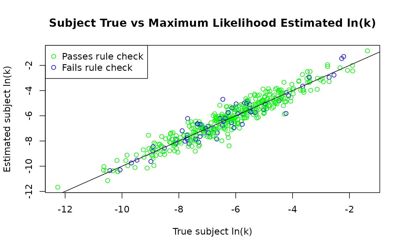
For example, the following code produces a plot of the true vs estimated subject $\log(k_{ic})$ parameters, with points colored by rule check result.

# Get a data frame consisting of one observation per subject, containing each
#  subject's true ln(k)
subj_true_ln_k <- sim_data %>%
  select(subj, true_ln_k, group) %>%
  unique()

# Merge the data frames containing the true subject ln_k values, estimated
#  subject ln_k values, and rule check results.
subj_ln_k_comp <- merge(subj_est_ln_k, subj_true_ln_k)
subj_ln_k_comp_wrc <- merge(subj_ln_k_comp, rule_check_results)

# Get the overall rule check result for each subject
subj_ln_k_comp_wrc$rc_pass <- subj_ln_k_comp_wrc$C1 & subj_ln_k_comp_wrc$C2

# Make a plot showing true vs estimated ln(k) for each subject,
#  coloring the points based on whether or not the corresponding subject
#  passed the rule check.
plot(x = subj_ln_k_comp_wrc$true_ln_k, y = subj_ln_k_comp_wrc$ln_k,
     col = ifelse(subj_ln_k_comp_wrc$rc_pass, "green", "blue"),
     main = "Subject True vs Maximum Likelihood Estimated ln(k)",
     xlab = "True subject ln(k)", ylab = "Estimated subject ln(k)")
abline(a=0, b=1)
legend("topleft", 
       legend = c(
         "Passes rule check",
         "Fails rule check"),
       col = c("green", "blue"), pch = 1)